Predicting a vehicles motion and direction using optical flow.

In this post we’ll explore the topic of optical flow. Optical flow has many useful application in computer vision such as structure from motion and video compression. Let’s see if it’s possible to use optical flow to predict a vehicle’s motion from a dash camera feed.

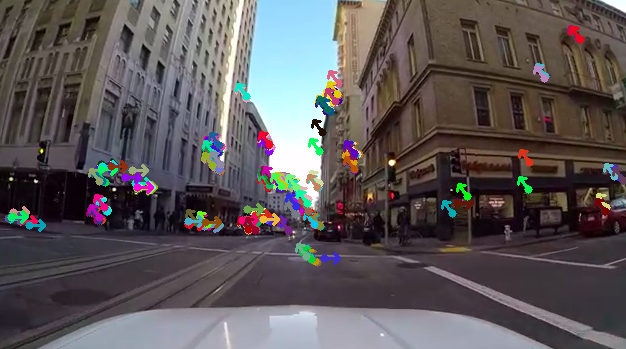
Thanks for the video: driving dash cam

Optical flow example

Optical Flow Algorithm

I decide to use Lucas–Kanade to calculate optical flow.

# Lucas–Kanade parameters
lk_params = dict(
  winSize  = (15,15), # window size for convolution
  maxLevel = 2,
  criteria = (cv2.TERM_CRITERIA_EPS | cv2.TERM_CRITERIA_COUNT, 10, 0.03))

kp1, st, err = cv2.calcOpticalFlowPyrLK(
  old_gray,   # Previous frame
  frame_gray, # Current frame
  kp0,        # Previous keypoints
  None,       # Current keypoints (None on initalization)
  **lk_params)

Collecting Features

I decided to use the ORB(Oriented FAST and rotated BRIEF) algorithm to collect features (or keypoints), from a video frame. ORB is the child of two different algorithms, which I’ll discuss briefly. Later, we will track the collected keypoints from ORB and use an optical flow algorithm called Lucas–Kanade to predict the vehicle’s motion and direction.

ORB uses FAST(Features from accelerated segment test ) to detect features; as you could have guessed from the name. The FAST feature detection algorithm is used to collect keypoints (i.e pixel regions that contain corners). I chose FAST because it preforms well with real-time video. FAST looks at a Bresenham circular region of 16 pixels and is able to detect corners quickly within a given threshold. It provides similar accuracy to the SIFT algorithm, but it accomplish it’s task in less time because it “checks” less pixels.

ORB uses BRIEF(Binary Robust Independent Elementary Features) to find feature descriptions.

Why combine FAST and BRIEF?

I’ll leave to explanation to Ethan Rublee

max_features = 400
detector = cv2.ORB_create(max_features)

# Later we'll use the ORB detector to collect
# keypoints (features) from a video frame.
keypoints, descriptors = detector.detectAndCompute(frame)

Predicting Motion and Direction

If we want to predict motion and direction, we’ll first need to find the mean angle of all the keypoints between two frames. After we have found the mean angle we can determine the direction from circular motion.

Calculating Mean Angle

We’ll use arctan to calculate the angle between keypoints. ${\theta } = arctan(\frac{y}{x})$

def get_angle(v1, v2):
    dx = v2[0] - v1[0]
    dy = v2[1] - v2[1]
    # arctan2 is the same as arctan, the difference
    # being x and y are separate parameters in arctan2
    return np.arctan2(dy, dx) * 180 / np.pi

When collecting angles between keypoints we will only collect points that are within a defined threshold. The threshold being, the distance between keypoints.

min_distance = 0.5
for kp1, kp2 in keypoints:
  if calc_distance(kp1, kp2) > min_distance:
    theta = calc_angle(kp1, kp2)
    angles.append(theta)

Defining Circular Direction and Motion

Now that we have found the mean angle, we can determine the motion and direction of the vechile. I will admit, this is going to be a bit hand-wavy.

Give the mean angle, we will define stationary motion to have 0 degrees. Forward motion will be greater than 0 degress and less than or equal to 180 degrees.

Try to imagine an object moving directly towards you. The angle between objects motion and the background plane is 90 degrees.

plane
 |       object    you
 | --------> *      *
 |

Using this intuition, we can determine if the object’s motion is more to the left or the right.

If the mean angle is greater than 0 degrees and less 90 degress, than the objects direction is more right.

If the mean angle is greater than 90 degrees and less 180 degress, than the objects direction is more left.

mean_angle = np.mean(angles)

if 180 >= mean_angle > 0:
  motion = 'forward'

if 90 > mean_angle > 0:
  direction = 'right'

if 180 > mean_angle > 90:
  direction = 'left'

Conclusion

This is by no means a perfect system for determining a vehicle’s motion, but it’s not a bad start.

Improvements/Enhancements

Calculate dense optical flow and only use keypoints found at the centroid of high density regions.
Try to predict the vehicle’s speed from the mean angle. In other words, compute the angular acceleration.
Find a motion dataset and train a spatiotemporal convolutional neural network, than compare the network’s prediction with the proposed optical flow algorithm.

Source code found here ⤧ Previous post Training on Large Scale Image Datasets with Keras

Predicting Vehicle Motion and Direction using Optical Flow